Related News
- 00
0000-00
What Affects Container Terminal Efficiency in Southeast Asia? - 00
0000-00
How to Use Maritime Trade Intelligence to Identify Promising Export Markets - 00
0000-00
Container Yard Optimization: How to Reduce Rehandles During Peak Operations - 00
0000-00
Shipping Rate Analytics for Terminals: Evaluating Data Quality and Coverage - 00
0000-00
Heavy Machinery Logistics for Ports: Planning Lifts, Routes, and Delivery Windows
0000-00
Automated Logistics Node Monitoring: How to Detect Distribution Hub Bottlenecks
A growing truck queue beside an idle quay crane does not necessarily mean the crane needs more capacity. Containers may be waiting for yard positions, vehicles may lack executable assignments, or a downstream transfer point may be unable to accept another load. Acting on the most visible queue can increase equipment activity without increasing completed moves.
Automated logistics node monitoring detects bottlenecks by linking arrival, service, departure, and equipment-state events across connected processes. The strongest signal is a sustained queue or rising wait time, combined with evidence explaining why the next transfer cannot happen. Start by separating processing time from waiting time, then trace blocked and starved states across neighboring nodes before changing dispatch rules or buying equipment.
Define the node around a transfer, not just a machine
A useful monitoring boundary follows the movement of a container, truck, or handling task. In a port-linked distribution hub, relevant nodes might include the gate inspection lane, container pickup position, yard crane work area, automated vehicle handover point, warehouse receiving dock, and outbound staging area.
Each node needs an identifiable entry condition and exit condition. For example, “truck inside terminal” is too broad to explain a pickup delay. Separate gate processing, travel to the assigned block, waiting for the handling position, lifting, and exit clearance. Otherwise, a slow document check and a congested yard lane disappear into the same turnaround metric.
Map the dependencies between these stages as well. A transfer may require an available receiving slot, a released container, an assigned vehicle, and permission from the control system. Monitoring only equipment availability misses these logical constraints.
- Ready queue: work that has arrived and satisfies the prerequisites for service.
- Held work: work present but awaiting documentation, inspection release, allocation, or another prerequisite.
- Active service: the handling or processing operation itself.
- Completed but blocked: work finished locally but unable to leave because the next node cannot accept it.
This separation prevents held containers from being mistaken for a physical capacity shortage and prevents a machine waiting for transport from being classified as simply idle.
Build a reliable event trail before adding alerts
The minimum useful record contains the job or container identifier, node identifier, event timestamp, event type, and source. Vehicle and equipment identifiers help connect handovers. Depending on the operation, events may come from the terminal operating system, warehouse management system, equipment controllers, gate readers, positioning systems, or dispatch software.
Capture physical events separately from administrative updates. A dispatch instruction is not proof that a vehicle arrived, and a completed task message may precede actual clearance of the transfer position. Where possible, retain both commanded and observed states so analysts can identify delays between instruction and execution.
Resolve three data problems early
- Clock misalignment: synchronize sources to a common time reference and measure remaining offsets. Incorrect event ordering can create negative travel times or false waiting periods.
- Identity gaps: reconcile container, task, and vehicle identifiers at handovers. Record split tasks, reassigned vehicles, and cancelled jobs explicitly rather than treating them as new arrivals.
- Missing or delayed messages: distinguish event time from ingestion time. Flag stale feeds and incomplete journeys instead of interpreting missing updates as equipment inactivity.
Duplicate messages also need removal. Retain raw events for investigation, but calculate operational metrics from validated transitions. When data quality deteriorates, the dashboard should show reduced confidence or an unknown state; a reassuring green indicator based on stale information is worse than an explicit gap.
Use metrics that expose the constraint
Total throughput remains necessary, but it usually confirms a problem after it develops. Pair completed transfers with queue growth, waiting-time distributions, and state durations. Calculate these by node, direction, work type, and operating period so that incompatible movements do not obscure each other.
Use queue conservation as a basic validation: ending queue equals starting queue plus arrivals minus departures, adjusted for cancellations, diversions, and reclassification. A persistent mismatch suggests missing events or inconsistent boundaries before it suggests an operational anomaly.
High utilization alone is not proof of a bottleneck. A busy crane may be serving demand efficiently, while a less busy transfer point limits the entire route through intermittent blocking. Likewise, average service time can remain stable while increasingly variable arrivals create longer queues.
Trace the delay beyond the visible queue
When an exception appears, follow the affected jobs across adjacent nodes. Compare the onset of queue growth with changes in service time, downstream occupancy, vehicle availability, and control-system states. The sequence of changes helps identify a likely cause, although it does not establish causation by itself.
A practical investigation sequence
- Validate the signal. Confirm that arrivals, departures, and equipment states are current. Check whether a new task mix or reporting change explains the apparent deterioration.
- Locate the waiting interval. Determine whether jobs wait before assignment, during travel, before service, or after service completion. Aggregate turnaround time cannot answer this.
- Inspect the next receiving node. Check usable positions, interlocks, access routes, and acceptance permissions. A machine unable to release its load is not necessarily processing slowly.
- Check upstream release behavior. Compare arrival bursts with appointments, vessel discharge sequences, and dispatch releases. Temporary overload can occur even when sustained capacity is adequate.
- Test the candidate explanation. Look for the same relationship across comparable operating periods and verify it against controller logs or field observations.
Consider a quay-to-yard transfer where crane waiting increases while automated vehicles cluster near a yard block. If yard handover positions remain occupied after lifting finishes, the constraint may be clearance or downstream placement rather than insufficient vehicle numbers. Releasing more vehicles could worsen lane congestion.
A different pattern calls for a different response: long crane waits, few vehicles approaching, and free receiving positions point toward dispatch starvation, routing delays, charging availability, or failed task assignment. Similar crane symptoms can therefore require opposite transport decisions.
Distinguish a demand surge from a persistent capacity limit
A temporary queue builds during a burst and drains once arrivals return to normal. A persistent constraint repeatedly accumulates ready work under comparable demand and cannot recover within the required operating window. Evaluate recovery behavior, not just the peak queue.
Build baselines around operational conditions: vessel work pattern, container type, yard block, shift configuration, equipment availability, and planned maintenance. Comparing a mixed inspection workload with unrestricted gate movements produces misleading thresholds. Where history is limited, begin with engineering estimates and label them provisional until observed cycles support refinement.
A node becomes a stronger capacity-investment candidate when ready demand persists, productive service is sustained, downstream acceptance is available, and avoidable interruptions have been addressed. Even then, examine variability and scheduling before equating nominal machine capacity with achievable route throughput.
Intermittent faults can impose an effective capacity limit despite acceptable average cycle times. Analyze stop frequency, recovery duration, and the backlog left after each interruption. A reliability improvement may address the constraint more directly than another handling asset.
Turn exceptions into actions with clear ownership
An alert should contain the affected node, waiting jobs, duration, data freshness, likely dependency, and responsible team. “High congestion” gives an operator little direction. “Ready queue rising while downstream receiving positions remain occupied” narrows the investigation without claiming an unverified root cause.
Use persistence rules and separate trigger and clear thresholds to avoid alarms repeatedly switching on and off. Tune these to the process cycle and available buffer, not to a universal interval. Escalate based on operational exposure, such as the oldest ready job, remaining staging capacity, or risk of starving a critical transfer.
- Dispatch starvation: investigate task eligibility, assignment logic, available vehicles, and route restrictions before increasing release rates.
- Downstream blocking: restore receiving capacity or meter upstream arrivals; do not simply accelerate the feeding equipment.
- Local service deterioration: inspect equipment condition, handling exceptions, and changes in workload composition.
- Administrative holds: route exceptions to the release or documentation owner rather than treating them as maintenance tasks.
Keep monitoring separate from safety-critical control. Automated changes to routing, release rates, or equipment coordination require approved limits, interlock preservation, rollback behavior, and validation by the relevant controls and operations teams.
Verify improvements across the full route
Start deployment on a bounded transfer chain with identifiable handovers and accountable operating teams. Establish event completeness, timestamp quality, and state definitions before expanding coverage. Run alerts in observation mode first, compare them with dispatch records and field conditions, and record false alarms as well as missed congestion.
For each corrective action, document the suspected mechanism and the expected observable change. Adjusting vehicle dispatch should change assignment or arrival gaps; clearing receiving positions should reduce blocked time. If the predicted interval does not improve, revisit the explanation rather than crediting unrelated throughput variation.
Evaluate comparable demand periods and track end-to-end completed moves, total waiting, downstream queue age, and buffer occupancy alongside the local metric. Include unfinished jobs so that moving difficult work outside the measurement window cannot create a false improvement.
An investment decision should follow the same evidence chain: a verified constraint, a proposed change that addresses it, and confirmation that neighboring nodes can absorb the additional flow. If local waiting falls but the next queue grows by a similar amount, the delay has moved—not disappeared.
Related News
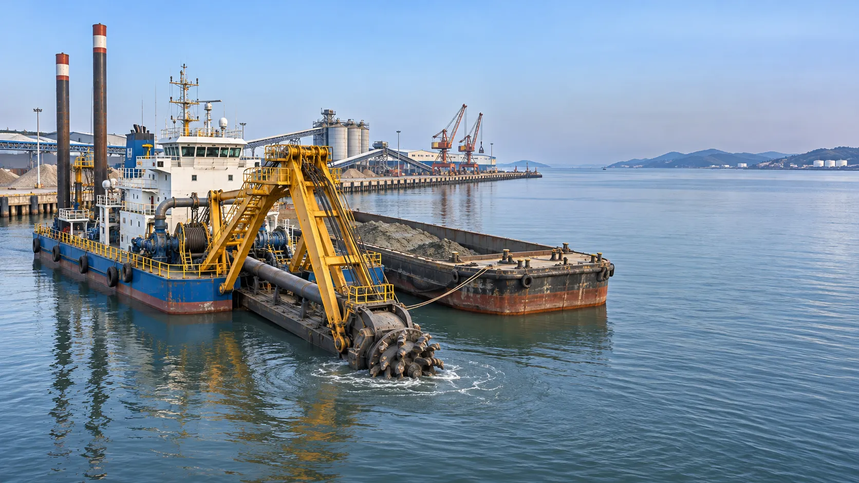
Marine Engineering Solutions for Dredging in Ports: Key Design Factors
Explore marine engineering solutions for dredging ports, from equipment selection and sediment management to safe navigation and survey verification.
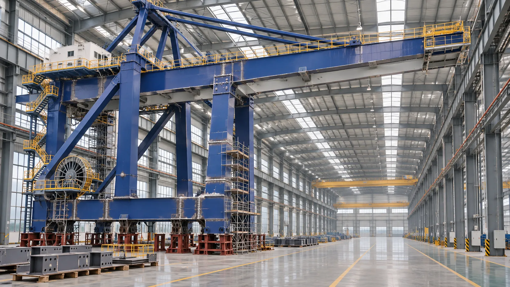
How to Evaluate a Quay Crane Factory: Capacity, Quality and Delivery
Evaluate a quay crane factory with confidence. Learn how to verify production capacity, quality controls, delivery plans, and lifecycle costs before you commit.
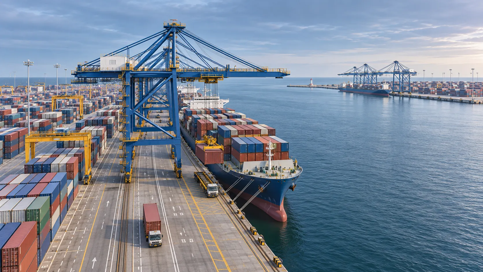
What Data Does a Smart Port Control Architecture Need to Operate?
What data is needed for a smart port control architecture? Discover the essential operational feeds, integration requirements and safety checks.
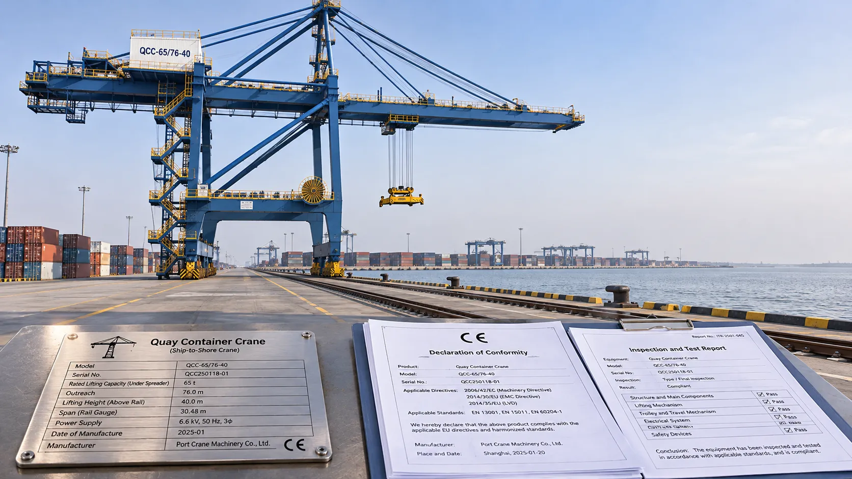
CE-Marked Quay Cranes: How to Verify Compliance Documents
Quay crane CE certified? Learn how to verify declarations, risk assessments and test records for the complete machine before acceptance.
Port Automation Systems in Latin America: Choosing the Right Solution
Explore port automation systems Latin America terminals can use to reduce congestion, assess integration risks, and choose the right solution with confidence.

Scalable Automated Port Systems: Planning for Terminal Capacity Growth
Discover how scalable automated port systems support phased terminal growth, reduce bottlenecks and guide smarter capacity investments.

Europe's Coastal Economies: Key Industries, Jobs and Climate Risks
Explore coastal economics in Europe: discover key industries and jobs, the climate risks they face, and how coastal communities can adapt.

Bulk Cargo Handling Equipment for Ports: Choosing by Cargo and Capacity
Choose bulk cargo handling equipment for ports with confidence. Compare cargo types, realistic throughput, equipment options, and lifecycle costs.
What Affects Container Terminal Efficiency in Southeast Asia?
Discover what affects terminal efficiency in Southeast Asia, from berth planning and yard congestion to inland access, and learn how to assess performance.